R Probability

A probability is a number that describes the “magnitude of chance” associated with making a particular observation or statement.

It’s always a number between 0 and 1 (inclusive) and is often expressed as a fraction.

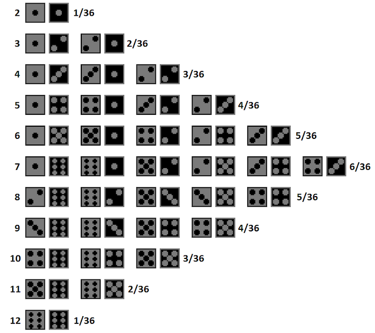
X.outcomes <- c(2:12)
X.prob <- c((1/36),(2/36),(3/36),(4/36),(5/36),(6/36),(5/36),(4/36),(3/36),(2/36),(1/36))
barplot(X.prob,ylim=c(0,0.20),names.arg=X.outcomes,space=0,xlab="x",ylab="Pr(X = x)", main = "probability distribution")

X.outcomes <- c(2:12)
X.prob <- c((1/36),(2/36),(3/36),(4/36),(5/36),(6/36),(5/36),(4/36),(3/36),(2/36),(1/36))
X.cumul <- cumsum(X.prob)
barplot(X.cumul,names.arg=X.outcomes,space=0,xlab="x",ylab="Pr(X <= x)", main = "cumulative probability distribution")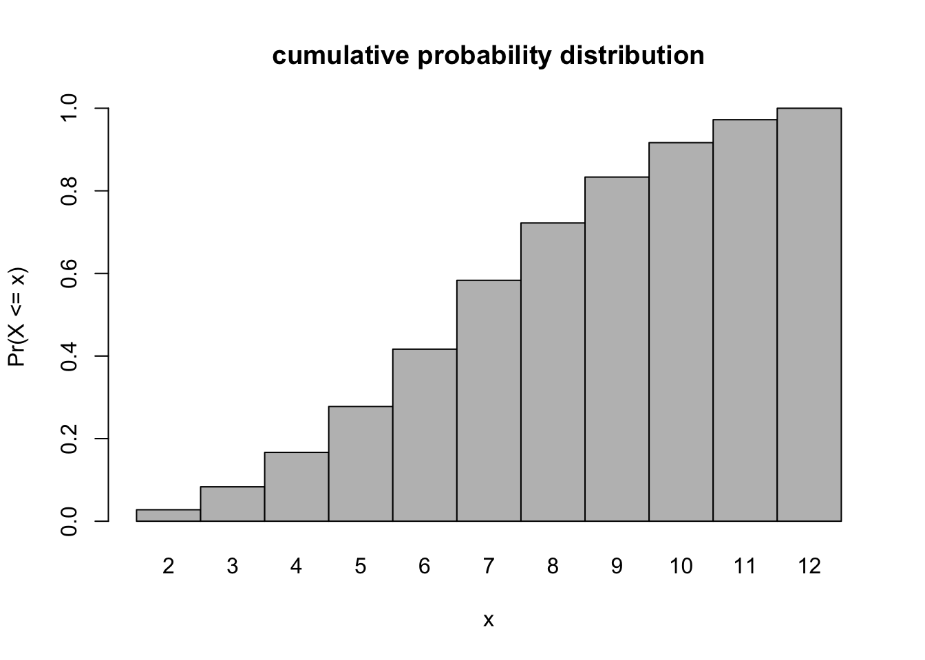

X.outcomes <- c(2:12)
X.prob <- c((1/36),(2/36),(3/36),(4/36),(5/36),(6/36),(5/36),(4/36),(3/36),(2/36),(1/36))
barplot(X.prob,ylim=c(0,0.20),names.arg=X.outcomes,space=0,xlab="x",ylab="Pr(X = x)", main = "probability distribution")
abline(v=c(0.5:10.5))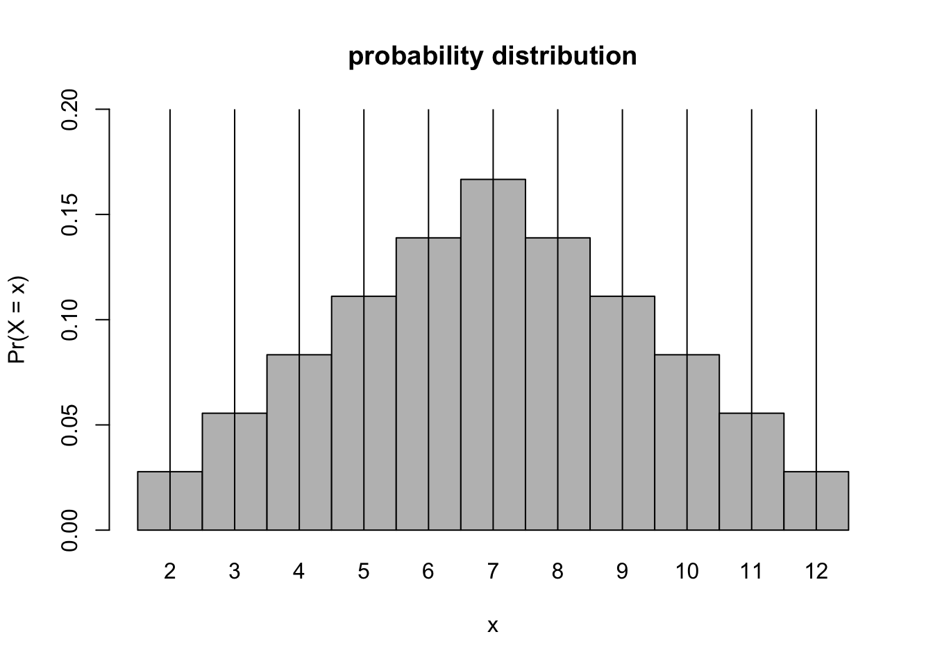

PDF - Probability Density Function

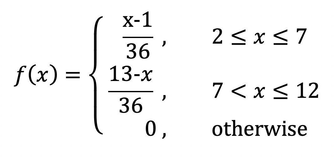
lower < 7 < upper

X >= 2  &  X <= 7
(X[lower] - 1)/36

X > 7 & X <= 12
13 - X[upper])/36

X.outcomes <- c(1,2,3,4,5,6,7,8,9,10,11,12,13)

lower <- X.outcomes >= 2 & X.outcomes <= 7
upper <- X.outcomes > 7 & X.outcomes <= 12

fx <- rep(0,length(X.outcomes))
fx[lower] <- (X.outcomes[lower] - 1)/36
fx[upper] <- (13 - X.outcomes[upper])/36

plot(X.outcomes,fx,type="l",ylab="f(x)", xlim = c(0,14), main = "probability density function")
abline(h=0,col="gray",lty=2)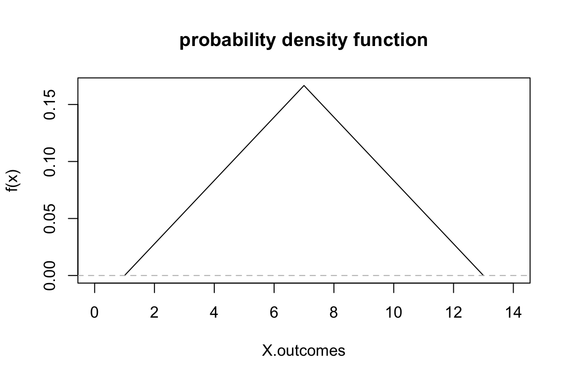

fx.specific <- (4.5-1)/36

fx.specific.area <- 3.5*fx.specific*0.5

fx.specific.vertices <- rbind(c(1,0),c(4.5,0),c(4.5,fx.specific))

plot(X.outcomes,fx,type="l",ylab="f(x)", xlim = c(0,14), main = "probability density function")
abline(h=0,col="gray",lty=2)
polygon(fx.specific.vertices,col="gray",border=NA)
abline(v=4.5,lty=3)
text(4,0.01,labels=fx.specific.area)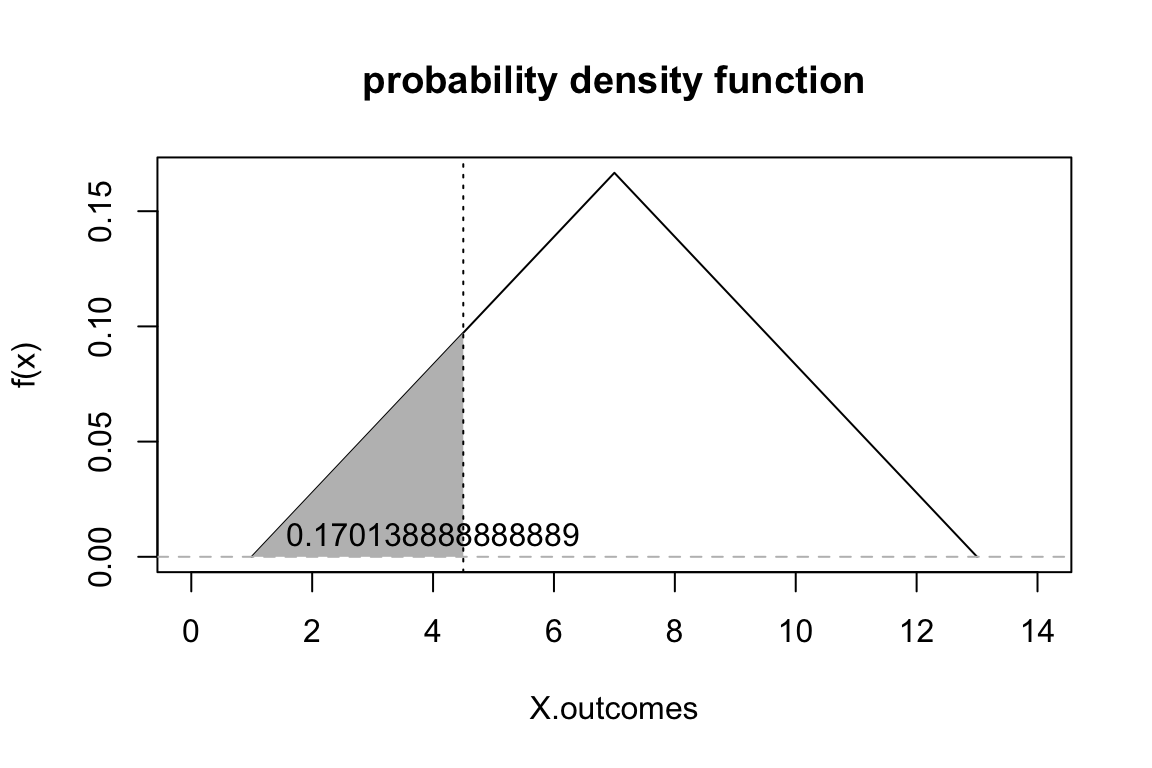

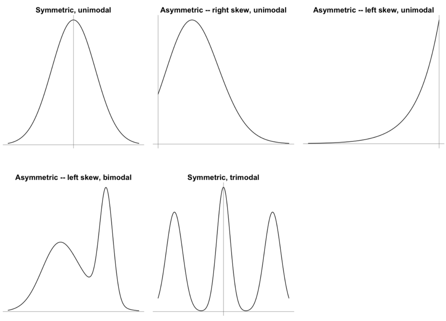
R - Probability - Shape

Symmetry : Draw a vertical line down the center, and it is equally reflected with 0.5 probability.
Skew : If a distribution is asymmetric, look at the “tail” of a distribution. Positive or right skew indicates a tail extending longer to the right of center.
Modality : Modality describes the number of easily identifiable peaks in the distribution of interest. Unimodal, bimodal, and trimodal…

station_data <- read.table("https://web.itu.edu.tr/~tokerem/18397_Cekmekoy_Omerli_15dk.txt", sep = ";", header = T)

table(station_data$temp)

## 
## 19.2 19.5 20.1 20.4 20.5 20.6 20.7 20.8 20.9   21 21.2 21.4 21.6 21.7 21.9 
##    1    1    1    4    6    4    2    6    2    1    2    3    1    2    1 
## 22.1 22.2 22.3 22.4 22.5 22.6 22.7 22.8   23 23.1 23.2 23.6 23.8 23.9 24.2 
##    1    5    3    3    8    7    1    1    2    1    3    1    2    2    2 
## 25.1 25.4 25.5 25.6 25.8 26.1 26.2 26.6 26.9 27.1 27.4 27.6 27.8   28 28.4 
##    1    1    1    1    1    1    1    1    1    1    1    1    1    1    2 
## 28.5 28.8   29 29.2 29.3 29.4 29.5 29.6   30 30.1 30.2 30.4 30.8 30.9   31 
##    1    1    2    2    2    1    1    1    1    2    1    4    1    3    1 
## 31.2 31.5 
##    1    1

df_temp_table <- data.frame(table(station_data$temp))
df_temp_table

##    Var1 Freq
## 1  19.2    1
## 2  19.5    1
## 3  20.1    1
## 4  20.4    4
## 5  20.5    6
## 6  20.6    4
## 7  20.7    2
## 8  20.8    6
## 9  20.9    2
## 10   21    1
## 11 21.2    2
## 12 21.4    3
## 13 21.6    1
## 14 21.7    2
## 15 21.9    1
## 16 22.1    1
## 17 22.2    5
## 18 22.3    3
## 19 22.4    3
## 20 22.5    8
## 21 22.6    7
## 22 22.7    1
## 23 22.8    1
## 24   23    2
## 25 23.1    1
## 26 23.2    3
## 27 23.6    1
## 28 23.8    2
## 29 23.9    2
## 30 24.2    2
## 31 25.1    1
## 32 25.4    1
## 33 25.5    1
## 34 25.6    1
## 35 25.8    1
## 36 26.1    1
## 37 26.2    1
## 38 26.6    1
## 39 26.9    1
## 40 27.1    1
## 41 27.4    1
## 42 27.6    1
## 43 27.8    1
## 44   28    1
## 45 28.4    2
## 46 28.5    1
## 47 28.8    1
## 48   29    2
## 49 29.2    2
## 50 29.3    2
## 51 29.4    1
## 52 29.5    1
## 53 29.6    1
## 54   30    1
## 55 30.1    2
## 56 30.2    1
## 57 30.4    4
## 58 30.8    1
## 59 30.9    3
## 60   31    1
## 61 31.2    1
## 62 31.5    1

barplot(df_temp_table$Freq/121,names.arg=df_temp_table$Var1)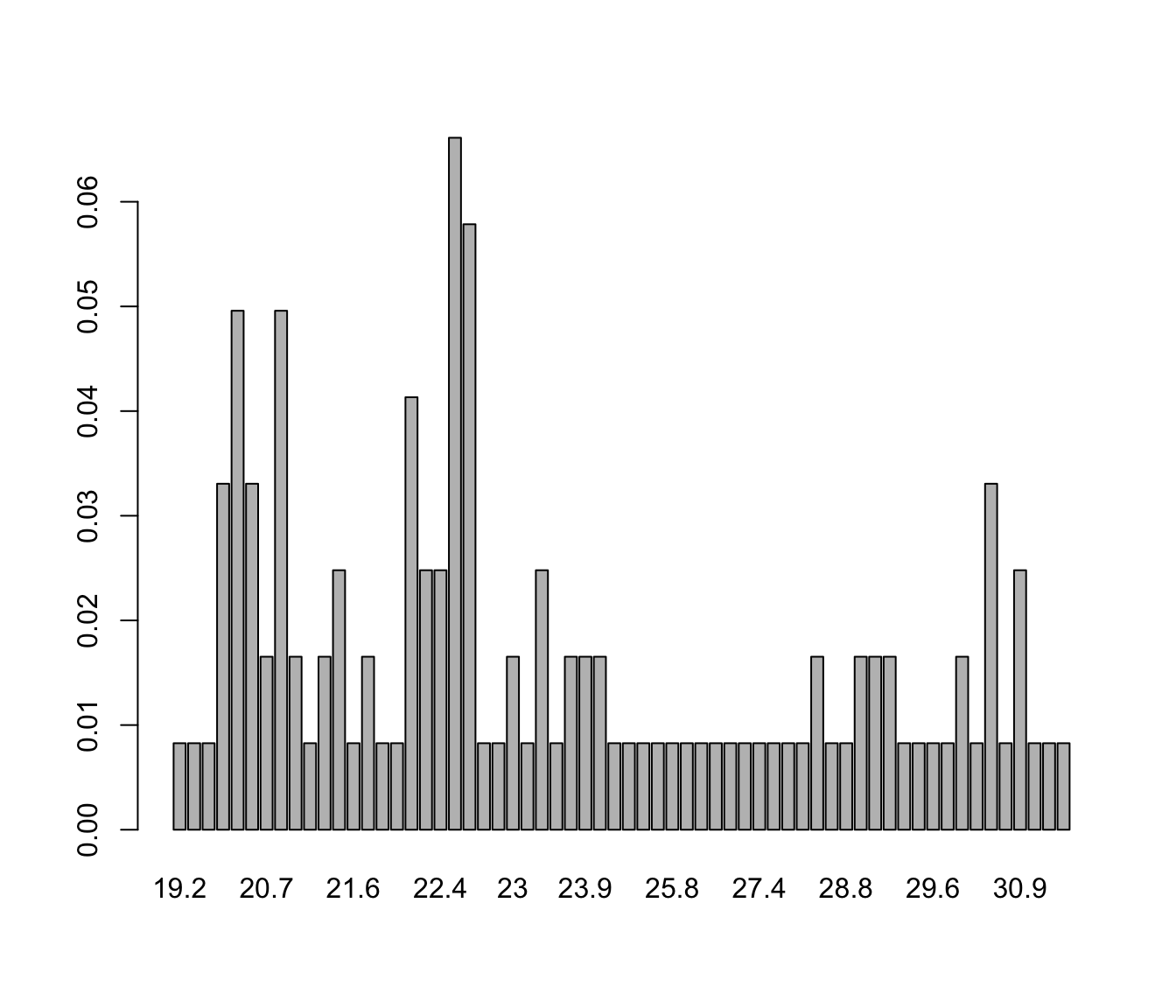

R - Common Probability Mass Functions

For discrete random variables

Bernoulli Distribution : has only two possible outcomes, such as success or failure.

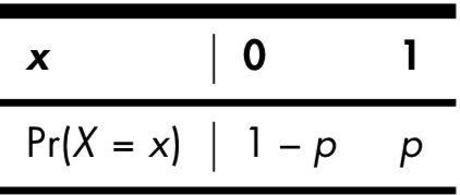
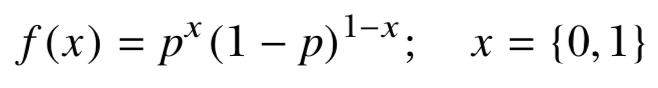
Bernoulli Distribution

x<-1
p <- 0.6

b_fx <- p^x*((1-p)^(1-x))

barplot(c(1-p,p),names.arg=c(0,1))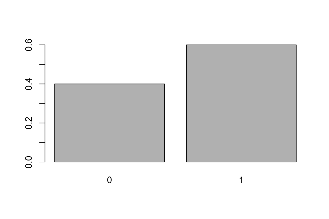

R - Common Probability Mass Functions

For discrete random variables

Binomial Distribution : The binomial distribution is the distribution of successes in n number of trials involving binary discrete random variables.

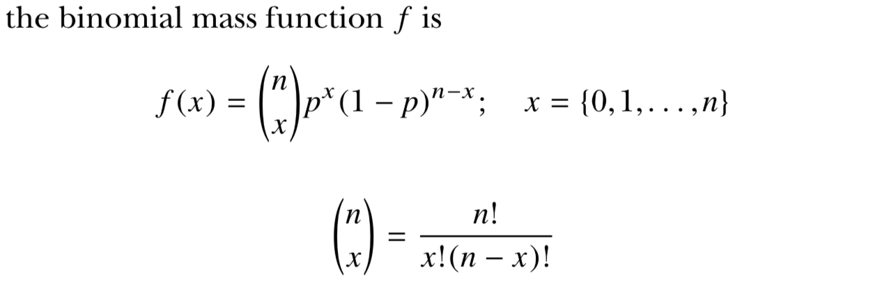
Binomial Distribution

There are four functions associated with Binomial distributions.

dbinom(x, size, prob)
pbinom(x, size, prob)
qbinom(p, size, prob)
rbinom(n, size, prob)
x is a vector of numbers.
p is a vector of probabilities.
n is number of observations.
size is the number of trials.
prob is the probability of success of each trial.

Binomial Distribution - dbinom

It is a density or distribution function.

x <- 1
size <- 8
prob <- 1/2
dbinom(x , size , prob)

## [1] 0.03125

x <- 4
dbinom(x , size , prob)

## [1] 0.2734375

x <- 0:8
dbinom(x , size , prob)

## [1] 0.00390625 0.03125000 0.10937500 0.21875000 0.27343750 0.21875000
## [7] 0.10937500 0.03125000 0.00390625

bin <- dbinom(x = 0:8 , size = 8 , prob = 0.5)
plot(x=0:8, y = bin)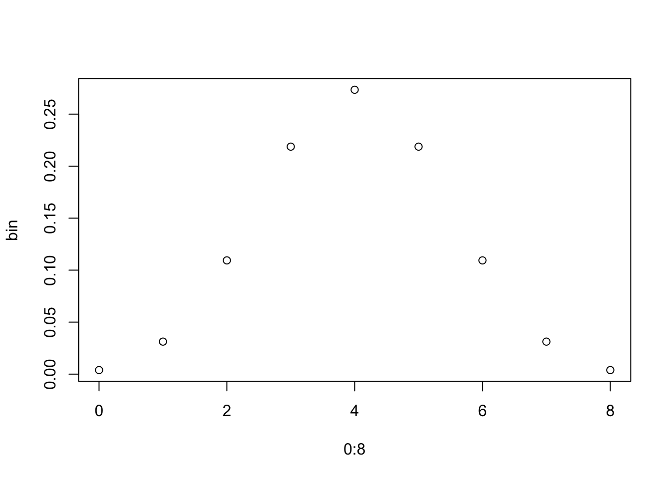

X.outcomes <- c(1:13)
X.prob <- c((0/36),(1/36),(2/36),(3/36),(4/36),(5/36),(6/36),(5/36),(4/36),(3/36),(2/36),(1/36),(0/36))
barplot(X.prob,ylim=c(0,0.20),names.arg=X.outcomes,space=0,xlab="x",ylab="Pr(X = x)", main = "probability distribution")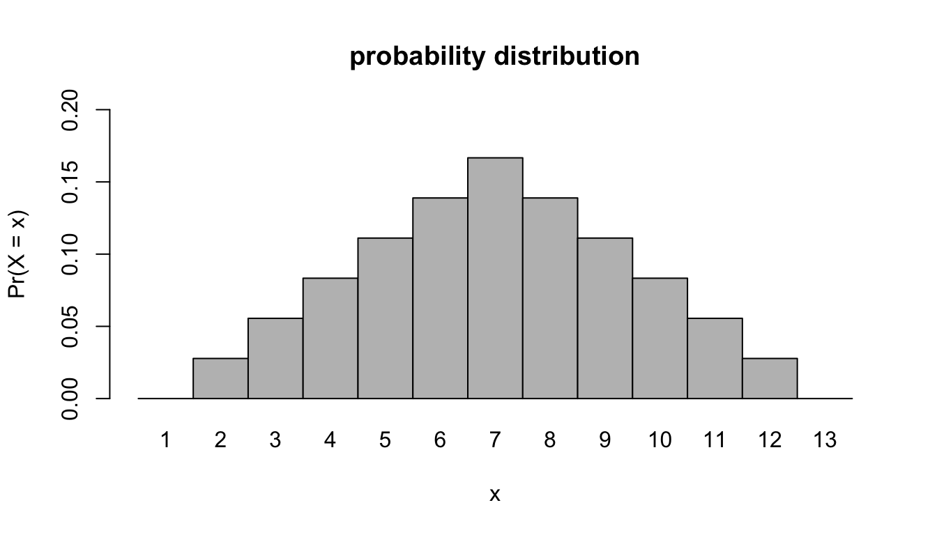

X.outcomes <- c(1:13)
X.prob <- c((0/36),(1/36),(2/36),(3/36),(4/36),(5/36),(6/36),(5/36),(4/36),(3/36),(2/36),(1/36),(0/36))
barplot(X.prob,ylim=c(0,0.20),names.arg=X.outcomes,space=0,xlab="x",ylab="Pr(X = x)", main = "probability distribution")

lines(dbinom(x = 0:12, size = 36, prob = 1/6), col= "red")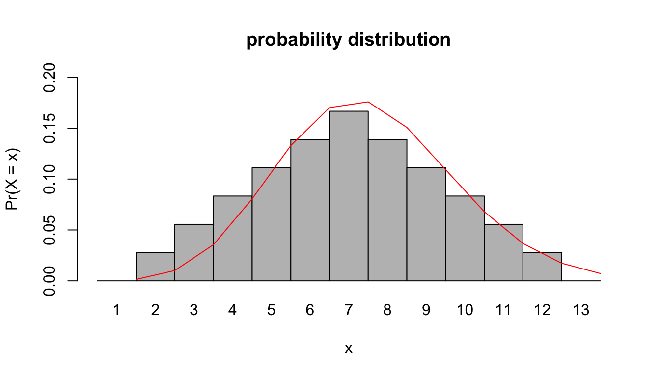

R - Common Probability Mass Functions

Poisson Distribution : important and rarely seen event.

λp should be interpreted as the “mean number of occurrences”

Poisson Distribution

There are three functions associated with Binomial distributions.

dpois(x, lambda)
ppois(q, lambda, lower.tail)
qpois(p, lambda, lower.tail)
rpois(n, lambda)
x : successes in a period
λ : the expected number of events
lower.tail = TRUE for left tail
q vector of quantiles
n number of random values to return
p vector of probabilities

plot(dpois(0:10,2.22),type = "o", col="red")
lines(dpois(0:10,4.22), type = "o", col = "blue")
lines(dpois(0:10,7.22), type = "o", col = "green")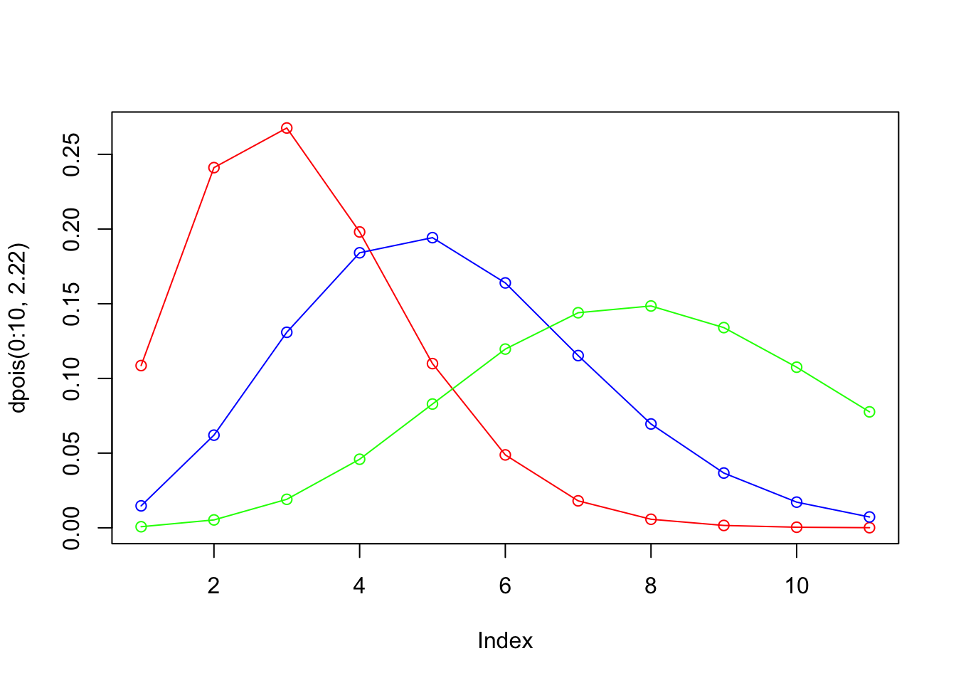

R - Common Probability Density Functions

- Uniform
- Normal
- Student’s t-distribution
- Exponential
- (gamma, beta, log-normal)

Uniform

The uniform distribution is a simple density function that describes a continuous random variable whose interval of possible values offers no fluctuations in probability.

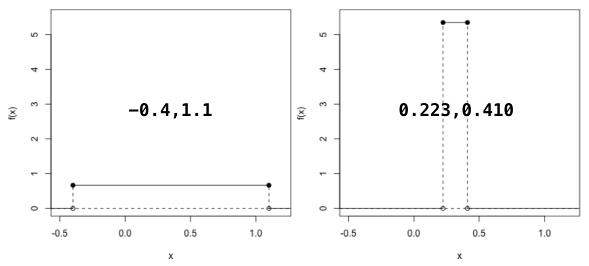
runif()
dunif()
punif()
qunif()

runif(n = 10,-0.4,1.1)

##  [1]  0.9105006  0.9006214 -0.2830141  0.3968495  0.9319934  0.2151849
##  [7]  0.5315867  0.8936403  0.7476632  0.6157447

r1 <- runif(n = 10,-0.4,1.1)
table(r1)

## r1
##  -0.398188538011163  -0.365233318158425  -0.154235270083882 
##                   1                   1                   1 
##  -0.144507477036677 -0.0904597032116726   0.159710376197472 
##                   1                   1                   1 
##   0.319758883002214   0.473805779847316   0.615361024765298 
##                   1                   1                   1 
##    1.03159253790509 
##                   1

t1 <- table(r1)

barplot(t1)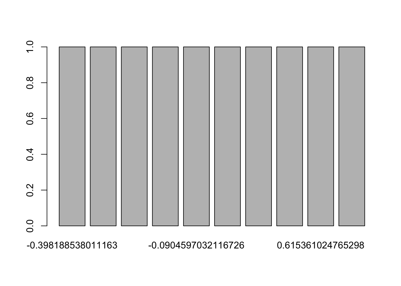

barplot(table(runif(n = 100,-0.4,1.1)))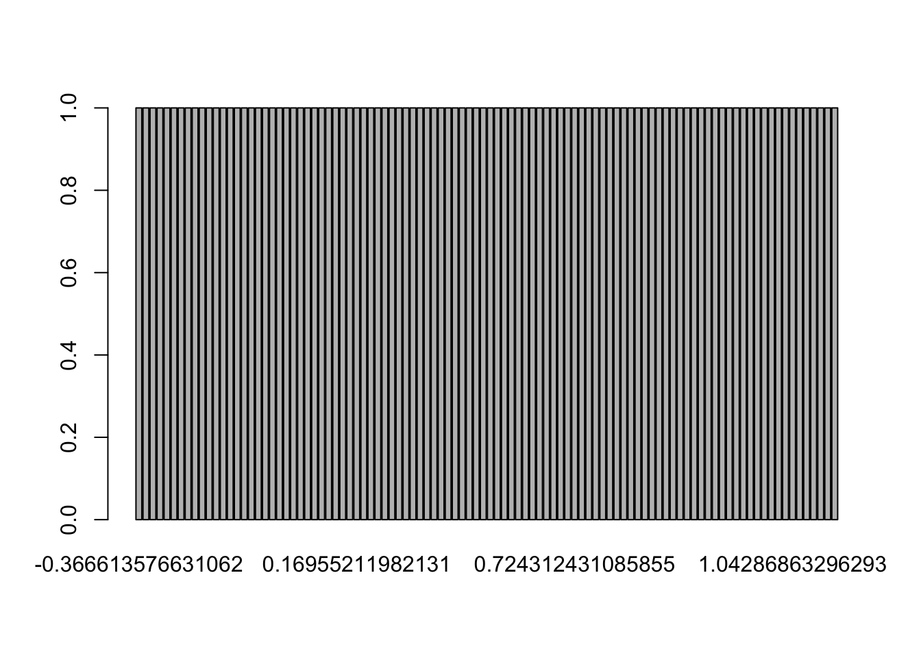

barplot(table(runif(n = 1000,-0.4,1.1)))

dunif(x=c(-2,-0.33,0,0.5,1.05,1.2),min=-0.4,max=1.1)

## [1] 0.0000000 0.6666667 0.6666667 0.6666667 0.6666667 0.0000000

d1 <- dunif(x=c(-2,-0.33,0,0.5,1.05,1.2),min=-0.4,max=1.1)
barplot(d1,names.arg=c(-2,-0.33,0,0.5,1.05,1.2))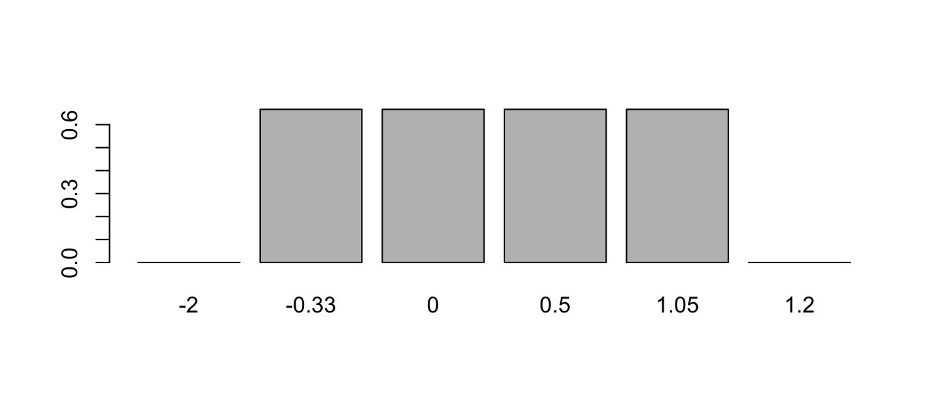

d2 <- dunif(x=c(-2,runif(998,-0.4,1.1),1.2),min=-0.4,max=1.1)
barplot(d2)

Characterized by a distinctive “bell-shaped” curve, it’s also referred to as the Gaussian distribution.

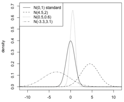
Normal

Standart Normal

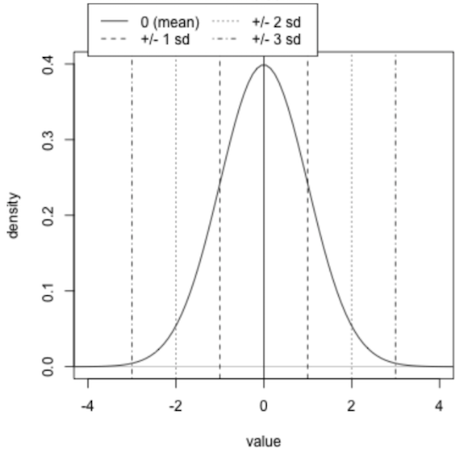
0.95 −2σ to +2σ and 0.99 −3σ tp +3σ

rnorm()
dnorm()
pnorm()

r1 <- rnorm(50,mean = 0, sd = 1)
r1

##  [1]  0.63191378  1.10297821  0.27035605  0.43025990  0.38154373
##  [6]  1.02321963  2.05586228 -2.75031632 -1.72808041  0.06489684
## [11]  1.58526306 -1.44759829  0.83461985 -0.18791933 -0.91344045
## [16] -0.73132253  0.74783234 -0.93842306 -0.29665193  0.68230962
## [21]  0.40157539  0.27835772  0.14834538  0.43097822  0.01371666
## [26]  2.08231240 -1.10497277 -0.29974305  0.51615597  0.15184775
## [31] -0.20615546  1.91093318  1.85923126  0.31599771 -0.23181942
## [36]  1.66971293 -0.84868078  0.58042305 -0.04699391  0.16519299
## [41] -1.54183815 -0.38155744 -1.32150222 -0.37041601  0.44044496
## [46]  1.13541998 -0.05831687 -0.30426056  1.34203867  0.46170168

plot(r1)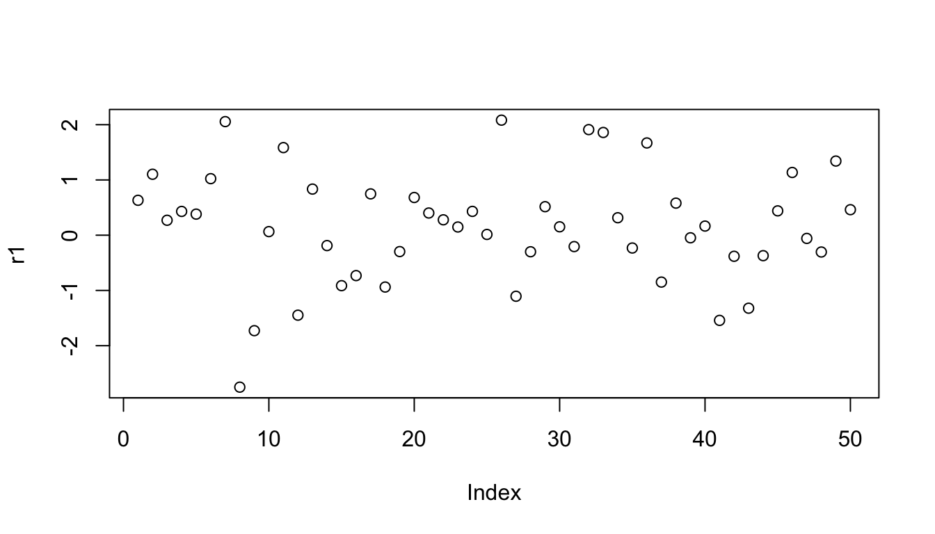

hist(r1)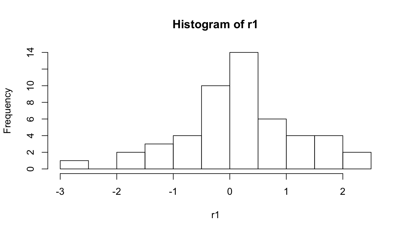

barplot(r1)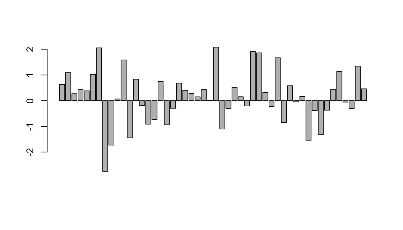

barplot(table(r1))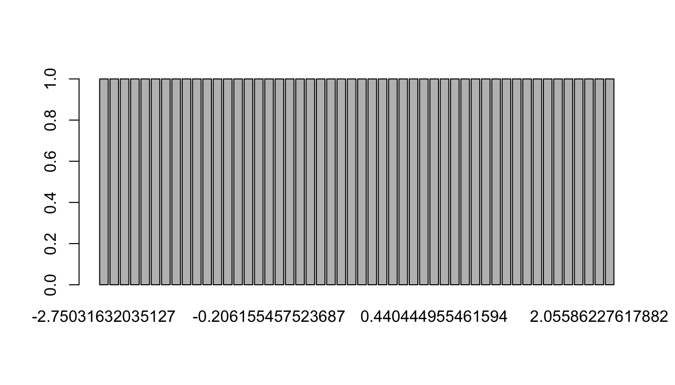

dnorm(r1, mean = 0, sd = 1)

##  [1] 0.326738197 0.217138692 0.384625660 0.363672943 0.370935775
##  [6] 0.236353258 0.048208333 0.009085655 0.089629615 0.398103072
## [11] 0.113554996 0.139916574 0.281609567 0.391960045 0.262862221
## [16] 0.305332219 0.301626694 0.256851430 0.381768942 0.316095233
## [21] 0.368037689 0.383782212 0.394576710 0.363560468 0.398904752
## [26] 0.045640902 0.216661090 0.381417203 0.349187229 0.394369338
## [31] 0.390554182 0.064262994 0.070841593 0.379513235 0.388365390
## [36] 0.098972903 0.278296532 0.337097190 0.398502006 0.393535935
## [41] 0.121532815 0.370933835 0.166606157 0.372490947 0.362063955
## [46] 0.209396059 0.398264484 0.380897192 0.162111255 0.358608952

fx3 <- dnorm(r1)

plot(r1,fx3)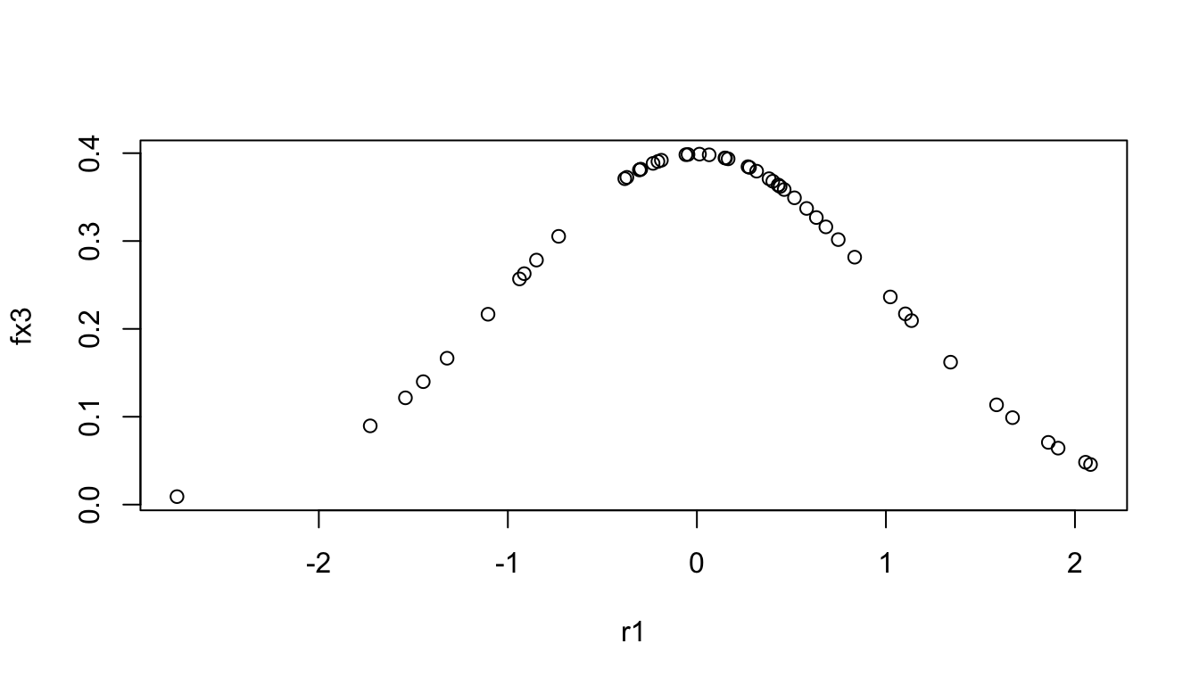

Practice : Write A Function for outliers

outliers

foo <- c(0.6,-0.6,0.1,-0.2,-1.0,0.4,0.3,-1.8,1.1,6.0)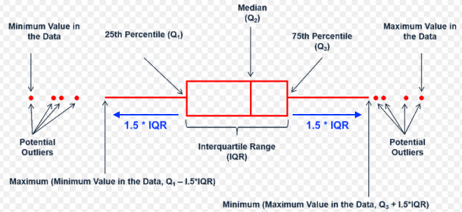

summary(foo)

##    Min. 1st Qu.  Median    Mean 3rd Qu.    Max. 
##   -1.80   -0.50    0.20    0.49    0.55    6.00

plot(foo,rep(0,10),yaxt="n",ylab="",bty="n",cex=2,cex.axis=1.5,cex.lab=1.5)
abline(h=0,col="gray",lty=2)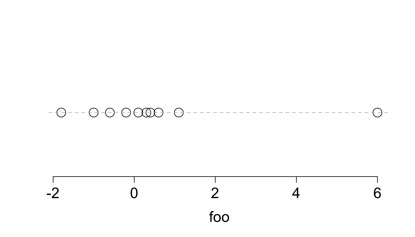

plot(foo,rep(0,10),yaxt="n",ylab="",bty="n",cex=2,cex.axis=1.5,cex.lab=1.5)
abline(h=0,col="gray",lty=2)
arrows(5,0.5,5.9,0.1,lwd=2)
text(5,0.7,labels="outlier?",cex=3)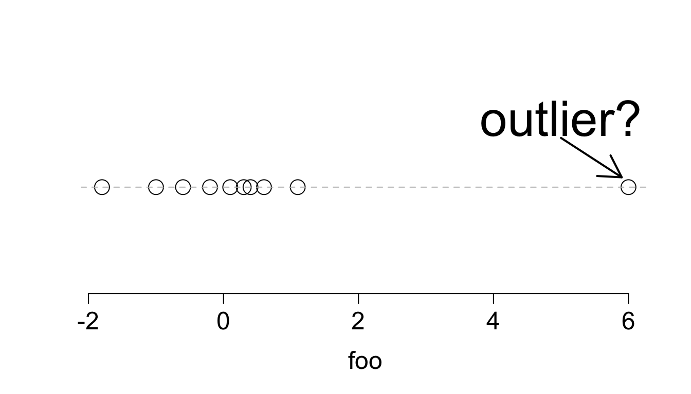

boxplot()

boxplot(foo)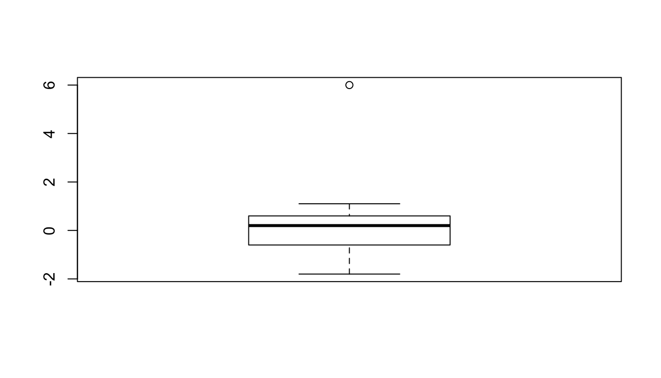

mean(foo)

## [1] 0.49

mean(foo[-10])

## [1] -0.1222222

Function

baz <- c(-0.3,0.9,2.8,2.3,1.2,12,-4.1,-0.4,4.1,-2.3)

Mean, Median, Range
Variance, Standart Deviation
Plot, hist
Barplot with table() function
summary() function
boxplot
if there is outliers, print

Condition for outliers is

OUTLIERS < MEAN-(3*IQR)

OUTLIERS > MEAN+(3*IQR)

baz <- c(-0.3,0.9,2.8,2.3,1.2,12,-4.1,-0.4,4.1,-2.3,1.2)

statistic_function <- function(baz) {

  
}

statistic_function <- function(baz) {
  print(c(mean(baz),"mean"))
  print(c(median(baz),"median"))
  print(c(range(baz),"range"))
  
}

statistic_function(baz)

## [1] "1.58181818181818" "mean"            
## [1] "1.2"    "median"
## [1] "-4.1"  "12"    "range"

statistic_function <- function(baz) {
  print(c(mean(baz),"mean"))
  print(c(median(baz),"median"))
  print(c(range(baz),"range"))
  print(c(var(baz),"var"))
  print(c(sd(baz),"sd"))

}

statistic_function(baz)

## [1] "1.58181818181818" "mean"            
## [1] "1.2"    "median"
## [1] "-4.1"  "12"    "range"
## [1] "17.2456363636364" "var"             
## [1] "4.15278657814682" "sd"

statistic_function <- function(baz) {
  print(c(mean(baz),"mean"))
  print(c(median(baz),"median"))
  print(c(range(baz),"range"))
  print(c(var(baz),"var"))
  print(c(sd(baz),"sd"))
  plot(baz)
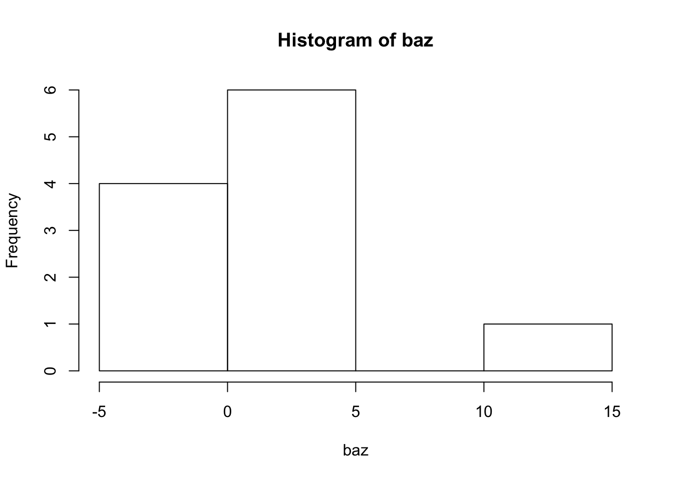
  hist(baz)
}

statistic_function(baz)

## [1] "1.58181818181818" "mean"            
## [1] "1.2"    "median"
## [1] "-4.1"  "12"    "range"
## [1] "17.2456363636364" "var"             
## [1] "4.15278657814682" "sd"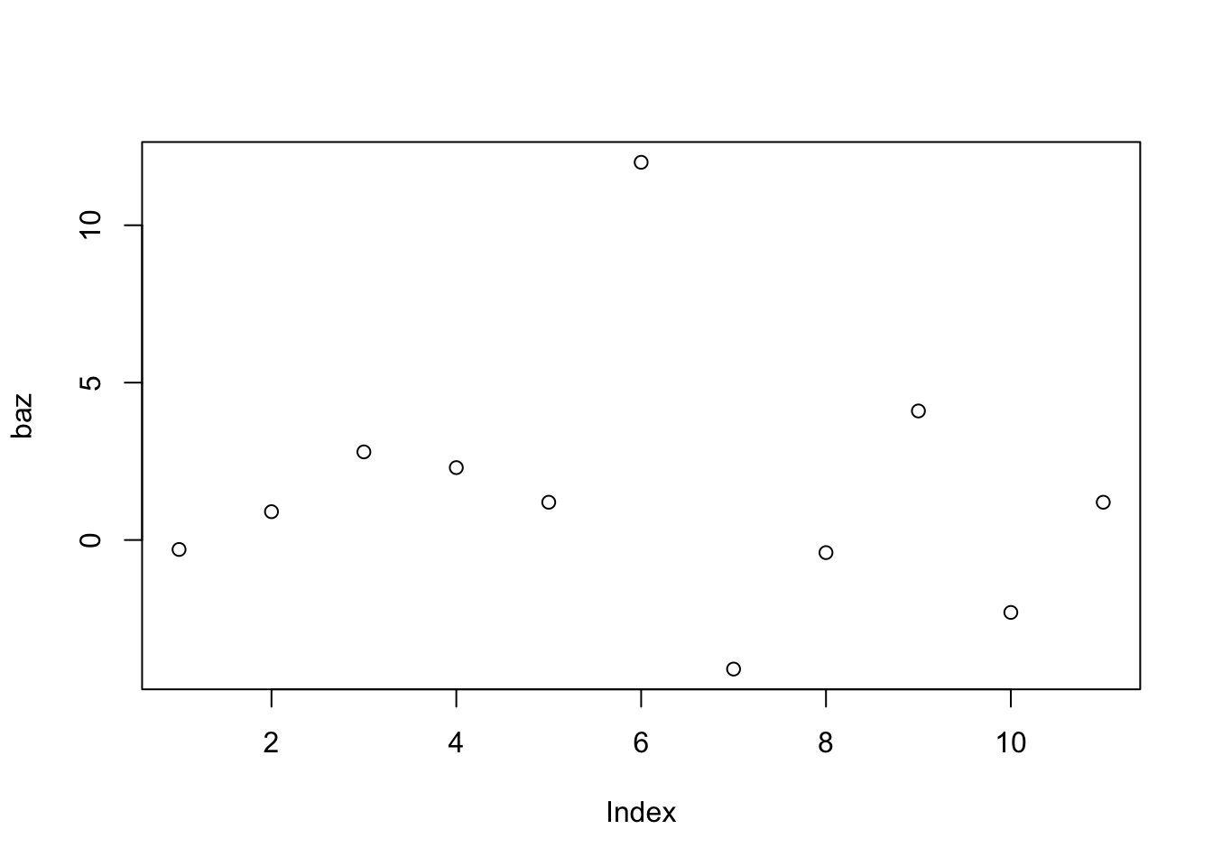

statistic_function <- function(baz) {
  print(c(mean(baz),"mean"))
  print(c(median(baz),"median"))
  print(c(range(baz),"range"))
  print(c(var(baz),"var"))
  print(c(sd(baz),"sd"))
  plot(baz)
  hist(baz)
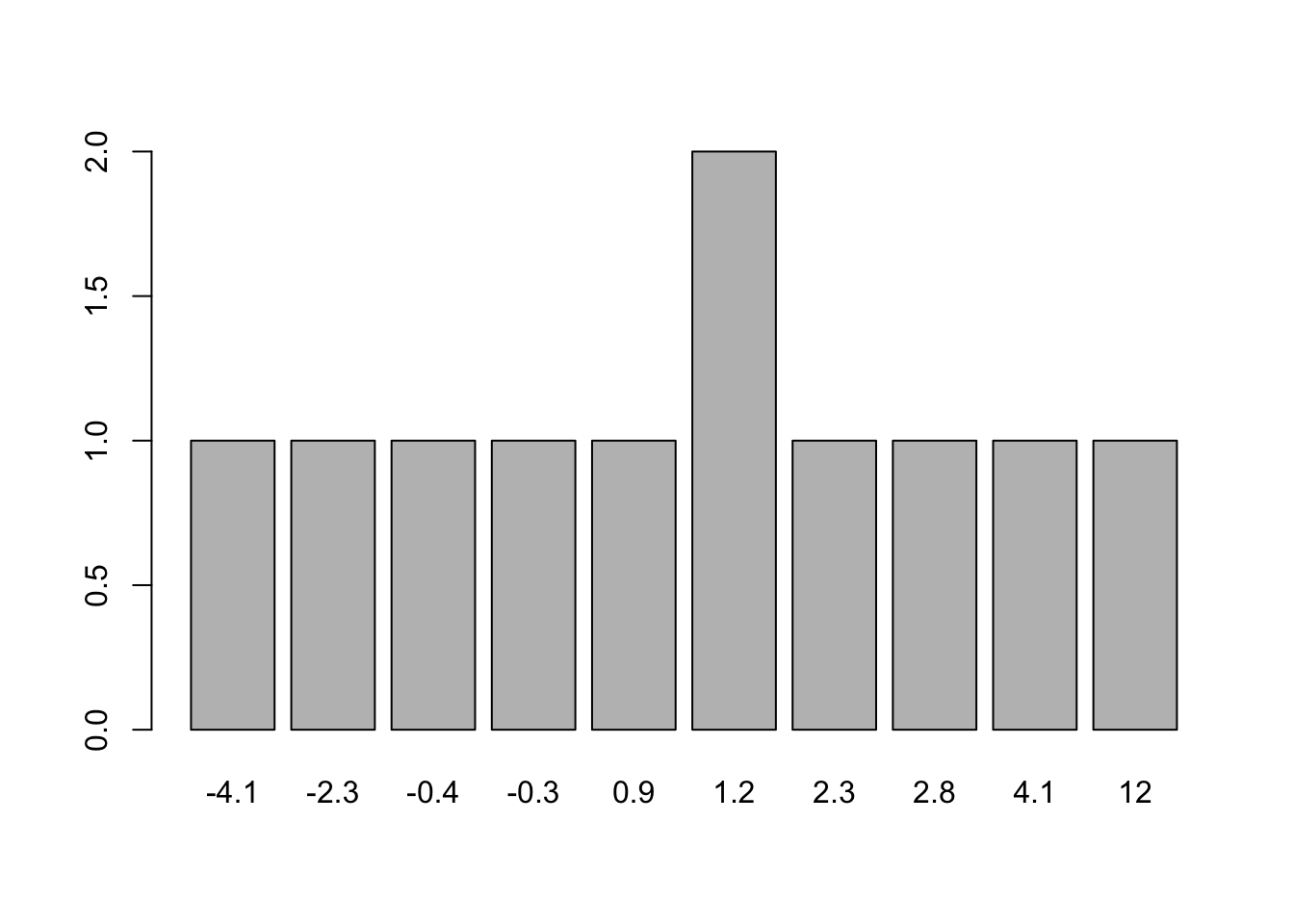
  barplot(table(baz))
  print(c(summary(baz),"summary"))
  boxplot(baz)
  
}

statistic_function(baz)

## [1] "1.58181818181818" "mean"            
## [1] "1.2"    "median"
## [1] "-4.1"  "12"    "range"
## [1] "17.2456363636364" "var"             
## [1] "4.15278657814682" "sd"

##               Min.            1st Qu.             Median 
##             "-4.1"            "-0.35"              "1.2" 
##               Mean            3rd Qu.               Max. 
## "1.58181818181818"             "2.55"               "12" 
##                    
##          "summary"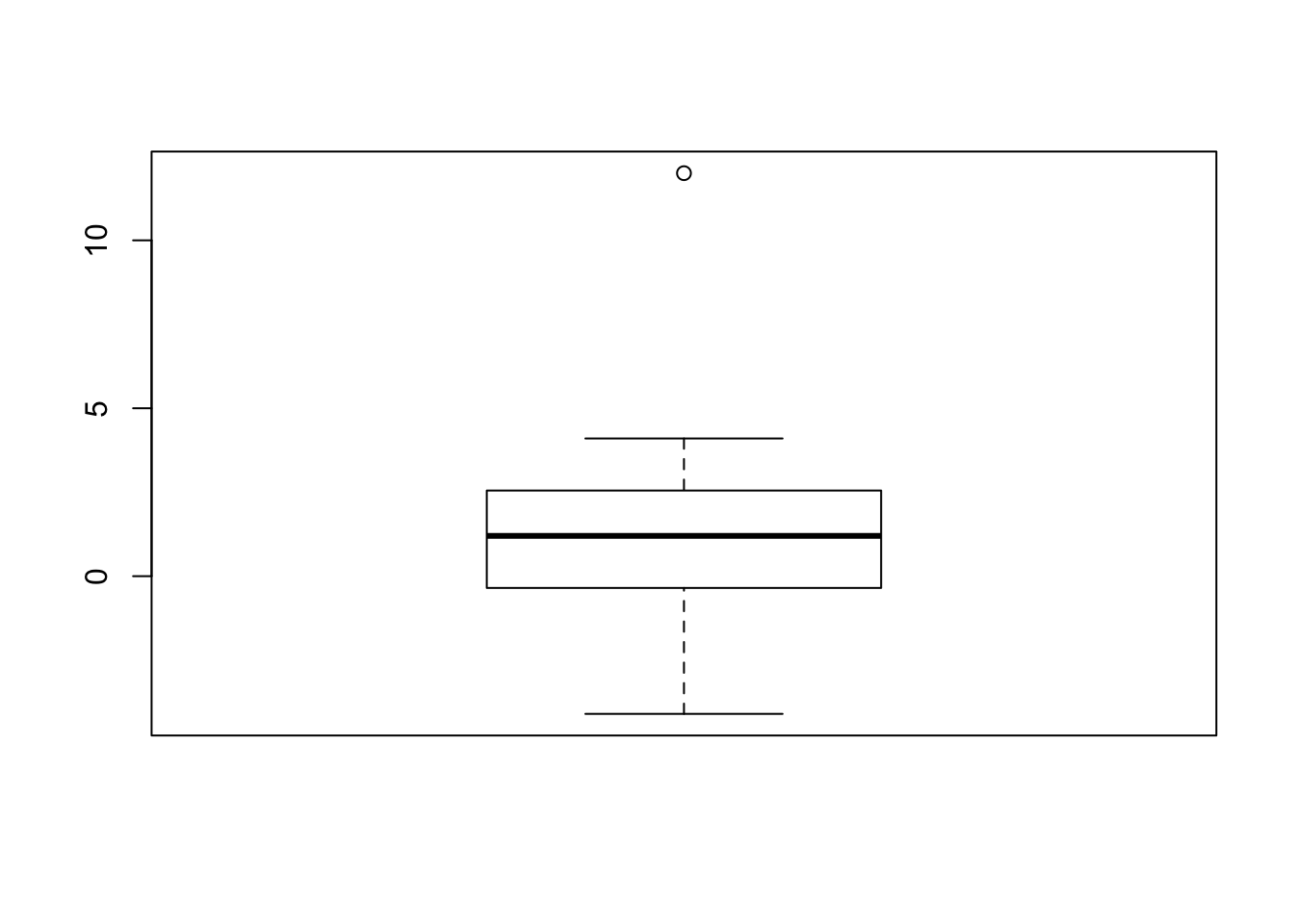

statistic_function <- function(baz) {
  print(c(mean(baz),"mean"))
  print(c(median(baz),"median"))
  print(c(range(baz),"range"))
  print(c(var(baz),"var"))
  print(c(sd(baz),"sd"))
  plot(baz)
  hist(baz)
  barplot(table(baz))
  print(c(summary(baz),"summary"))
  boxplot(baz)
  for (i in 1:length(baz)) {
      if (baz[i]<mean(baz)-3*IQR(baz) | baz[i]>mean(baz)+3*IQR(baz)) {
        print("there is outliers")
        print(c(baz[i] , "outlier") )
        print(which(baz==baz[i]))
      }
  }
}

statistic_function(baz)

## [1] "1.58181818181818" "mean"            
## [1] "1.2"    "median"
## [1] "-4.1"  "12"    "range"
## [1] "17.2456363636364" "var"             
## [1] "4.15278657814682" "sd"

##               Min.            1st Qu.             Median 
##             "-4.1"            "-0.35"              "1.2" 
##               Mean            3rd Qu.               Max. 
## "1.58181818181818"             "2.55"               "12" 
##                    
##          "summary"

## [1] "there is outliers"
## [1] "12"      "outlier"
## [1] 6